In this article we will find stocks and ETFs that have high levels of autocorrelation, and try to determine whether that data can be used to build a trading strategy.

Related articles:

• Getting started: using Python to find alpha [2021]
• Do CAPM efficient portfolios really outperform random ones? [2021]
• Do Equities Really Follow a Normal Distribution? [2021]

Using the partial autocorrelation function

To determine whether there is autocorrelation — and if so, how much there is — we use the PACF, or Partial Autocorrelation Function. This function determines the correlation of a time series with itself a number of periods prior.

In order to illustrate, we will use the SPY ETF. It’s very simple to run the PACF in Python. In the following code, we load the SPY data and plot the PACF:

data = pd.read_csv("spy.csv")
data.index = pd.to_datetime(data['date'])
data = data['adj_close'].pct_change()
data = data['2018-01-01':]
plot_pacf(data)

The resulting plot looks like this:

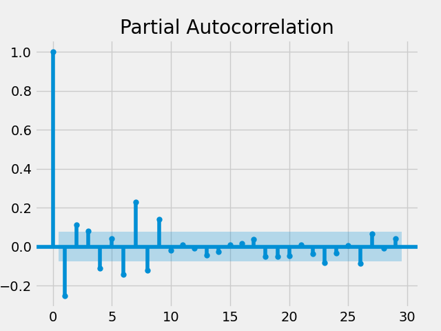
This plot shows the degree of autocorrelation between the return of SPY today and the return of SPY n days back, where n is the x axis.

From this plot, we see that the autocorrelation between the SPY returns on a given day and the returns on the previous day (where the x axis = 1) is around -.25. We can also see that the correlation between the SPY returns on a given day and two days prior is around .1.

The light blue bands tell us whether this correlation is statistically significant. If a value is outside of the band, it is statistically significant. Otherwise, it is not and we should ignore it. Note that for nearly all days after day 9, the values are not statistically significant.

As an aside, we could also use the plot_acf function, which would give us this plot:

Note that the values in the second plot are higher than those in the previous plot. The PACF ignores indirect correlations, whereas the ACF includes them.

For instance, if the return at day t is correlated with the return at day t-1, and the return at day t-1 is correlated with the return at day t-2, then the ACF shows a correlation between days t and t-2. The PACF would not show this correlation since it is already taken into account in the correlation between days t and t-1.

Determining autocorrelation for the universe of stocks and ETFs

We can now run a test for correlation on our entire dataset, and look for the most correlated tickers. Since we don’t want to plot every ticker, we will replace plot_pacf with pacf. Note that pacf returns the correlation as well as a shifted confidence interval. If that interval contains 0, it means that the result is statistically significant.

Here’s our code to do this. We use stock data and ticker info from Quandl:

try: 
    ticker_data = pd.read_csv("tickers.csv")
except FileNotFoundError as e:
    pass


ticker_data = ticker_data.loc[((ticker_data['table'] == 'SF1') | (ticker_data['table'] == 'SFP')) & (ticker_data['isdelisted'] == 'N') & (ticker_data['currency'] == 'USD') & ((ticker_data.exchange == 'NYSE') | (ticker_data.exchange == 'NYSEMKT') | (ticker_data.exchange == 'NYSEARCA') | (ticker_data.exchange == 'NASDAQ'))]

results = pd.DataFrame(columns=['ticker','l1', 'l2', 'l3', 'l4', 'l5'])

for t in ticker_data['ticker']:
    if t == 'TRUE': continue
    try:
        data = pd.read_csv(t + ".csv", 
                            header = None,
                            usecols = [0, 1, 12],
                            names = ['ticker', 'date', 'adj_close'])
    
        data.index = pd.to_datetime(data['date'])
        data = data['adj_close'].pct_change()
        data = data['2014-01-01':]
        
        if (len(data) < 15):
            continue
        
        [res,ci] = pacf(data, nlags=5, alpha=.05)
        for j in range(1, 6):
            if res[j] > 0:
                res[j] = ci[j][1]
            else:
                res[j] = ci[j][0]
            

        results.loc[len(results)]= [t] + res[1:].tolist()
    except FileNotFoundError:
        pass

The pacf function returns a list of results and a confidence interval for each one. The function is written in such a way that the confidence interval is shifted by the result. Therefore, we can simply look at the distance of the boundary of the confidence interval from 0.

After running this code, we have a results DataFrame which contains 5 days of autocorrelations by ticker. Let’s look at the tickers with the highest day 1 correlation:

     ticker        l1        l2        l3        l4        l5
2172   KODK  0.438201 -0.250540  0.055132 -0.070692  0.081623
6496    TFI  0.349147  0.149567 -0.121855 -0.338199 -0.049053
6113    PZA  0.345831 -0.119451  0.062336 -0.238694 -0.194027
5450   IGSB  0.333443 -0.055681  0.115657 -0.131023  0.083334
6620   VCSH  0.332864  0.079902  0.062387 -0.127547  0.062723
5372   HYLS  0.317959  0.202700  0.050186 -0.166055 -0.144543
5779   MINT  0.316034  0.065577  0.222451  0.136379 -0.052238
5924    NYF  0.313376  0.201103 -0.186961 -0.245647 -0.130453
909    CNTY  0.294874  0.139255 -0.179101 -0.161458 -0.053789
3959   UONE  0.284736 -0.055110  0.184917 -0.161995  0.087707
5157   FTSL  0.278337  0.207237  0.119671 -0.056239 -0.072306
4382    BAB  0.273436 -0.236646 -0.196171  0.107094  0.127834
3337    RWT  0.264686 -0.163005 -0.170003  0.051506 -0.189675
1253    EFC  0.261613 -0.078656 -0.181922  0.171257 -0.297007
5801   MORT  0.257654  0.056583 -0.135256  0.086857 -0.144170
2687   NMFC  0.251705  0.145104 -0.101689 -0.267327 -0.114394
6354   SLQD  0.250446  0.134402  0.089237 -0.232306  0.124600
6401   SPIB  0.248056  0.092669  0.083518 -0.157038  0.090045
1922   IBIO  0.244930 -0.175744  0.098071  0.094607 -0.051653
23      ABR  0.241716  0.070130 -0.104922 -0.090260 -0.091360

Let’s look at some of these tickers individually. Here is the partial autocorrelation plot for KODK:

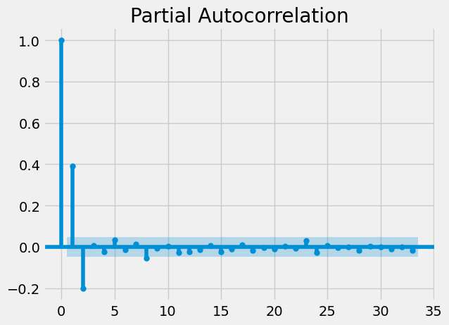
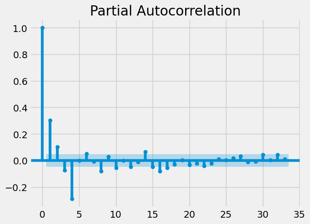
We can see that there is an extremely strong one day lagged autocorrelation for this stock. Let’s look at another (TFI):

Is there autocorrelation of stock returns on larger time scales?

Now we will look at monthly time scales. We adjust our code to resample by business month:

try: 
    ticker_data = pd.read_csv("tickers.csv")
except FileNotFoundError as e:
    pass


ticker_data = ticker_data.loc[((ticker_data['table'] == 'SF1') | (ticker_data['table'] == 'SFP')) & (ticker_data['isdelisted'] == 'N') & (ticker_data['currency'] == 'USD') & ((ticker_data.exchange == 'NYSE') | (ticker_data.exchange == 'NYSEMKT') | (ticker_data.exchange == 'NYSEARCA') | (ticker_data.exchange == 'NASDAQ'))]

results = pd.DataFrame(columns=['ticker','l1', 'l2', 'l3', 'l4', 'l5'])

for t in ticker_data['ticker']:
    if t == 'TRUE': continue
    try:
        data = pd.read_csv(t + ".csv", 
                            header = None,
                            usecols = [0, 1, 12],
                            names = ['ticker', 'date', 'adj_close'])
    
        data.index = pd.to_datetime(data['date'])
        data = data['adj_close'].pct_change()
        data = data['2014-01-01':]
        
        if (len(data) < 15):
            continue
        
        [res,ci] = pacf(data, nlags=5, alpha=.05)
        for j in range(1, 6):
            if res[j] > 0:
                res[j] = ci[j][1]
            else:
                res[j] = ci[j][0]
            

        results.loc[len(results)]= [t] + res[1:].tolist()
    except FileNotFoundError:
        pass

Here we have the top monthly auto-correlated tickers, with the last 5 months’ lag showing.

     ticker        l1        l2        l3        l4        l5
4155    BIL  1.062948  0.671578  0.406545  0.296207  0.267860
2030   KIRK  0.741970  0.273084 -0.483974  0.308310  0.236260
5896    SHV  0.693188  0.515499  0.327983  0.318500  0.461331
1694   HEAR  0.647345  0.263520 -0.328804 -0.238193 -0.389770
689     CCV  0.587156  0.310129  0.583598 -0.552379 -0.401946
3365   SPNV  0.557627  0.260339 -0.302074  0.403751  0.240059
5593    PFH  0.555545  0.234674 -0.280491 -0.271333  0.283133
3779   VBIV  0.555185 -0.345410 -0.337042 -0.324246  0.310560
3194   SCOR  0.545700 -0.297076 -0.406047 -0.368039 -0.321558
5496    NMZ  0.543346 -0.437787 -0.305792 -0.396759 -0.256477
125     AIM  0.538091  0.280120 -0.369887 -0.329034 -0.257873
2730   OSTK  0.537406  0.276835  0.495272 -0.391599 -0.367689
5495    NMY  0.533144 -0.401574  0.255636 -0.376926 -0.260971
1683   HCAP  0.530111 -0.391663  0.304328 -0.269658  0.380937
2603   NVAX  0.529282  0.264697  0.377803  0.306428  0.308998
5430    MUJ  0.516649 -0.255428 -0.330438 -0.346465  0.221122
119    AHPI  0.514086 -0.409486  0.222293  0.227159 -0.263185
4181    BNY  0.508837 -0.338257  0.313896 -0.415420  0.336402
2810   PEIX  0.503102  0.337251  0.265116 -0.280291 -0.313332
2056   KOPN  0.500044  0.364696 -0.384475  0.236588 -0.332640

Let’s plot some of these individually.

Can autocorrelation of stock returns be used in a trading strategy?

In this section we will examine whether we can use autocorrelation of stock returns in order to build a profitable trading strategy. For simplicity, we will assume that our carrying fees and trading costs are zero (though in practice, these could affect the profitability significantly).

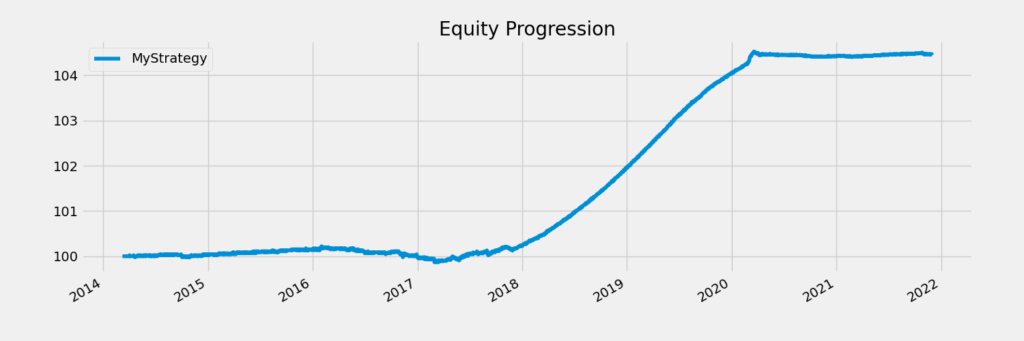
Let’s start with a monthly strategy using the most autocorrelated ETF we found. We will run a simple strategy using BIL, where we buy the ETF at closing whenever the previous month had a positive return. We will short the ETF if the previous month had a negative return.

We use the bt package in Python to run this strategy, and get the following result:

Total Return         4.45%
Daily Sharpe         2.37
Daily Sortino        4.15
CAGR                 0.56%
Max Drawdown         -0.35%
Calmar Ratio         1.61

This is a pretty good result considering the low volatility. Here is a chart of our returns:

Unfortunately, if we factor in short selling and trading costs, this trade will likely become a loser. Let’s try another ticker. MUJ is a municipal bond fund, which exhibits low volatility. If we run the backtest on this ticker, we get:

Total Return         50.29%
Daily Sharpe         0.55
Daily Sortino        0.80
CAGR                 5.41%
Max Drawdown         -28.19%
Calmar Ratio         0.19

A 50% return contrasts with the 5-10% return you would have received with a buy and hold strategy. So this is profitable, but we would have done much better if we just invested in the S&P500.

Conclusion

So can autocorrelation predict stock returns? The answer is: somewhat. We can find certain tickers that are reasonably autocorrelated, and those are somewhat predictable. However, building a successful trading strategy using just autocorrelation is very difficult — if not impossible.