
Does pairs trading still work (if you’re not a hedge fund)? [2021]
![Does pairs trading still work (if you’re not a hedge fund)? [2021]](https://firemymoneymanager.com/wp-content/uploads/2021/01/screenshot-2021-01-26-10-15-40-800x391.png)
In this article, we will look at a popular algorithm for hedge funds and high-frequency traders called pairs trading. In its most basic form, you select a pair of stocks that historically move together and trade when they diverge. The expectation is that as they return to a normal state, you will make money.
This is still a workable strategy for high frequency hedge fund traders who can co-locate giant server farms in exchange datacenters, but can it still work for average traders who don’t have these resources? Or are all of these statistical arbitrage opportunities gone by the time an average trader can execute? Can this strategy be run at a daily/weekly frequency anymore or does it have to be run in milliseconds?
We will run some tests on the basic strategy to see if it can work today.
Historical profitability of pairs trading
Pairs trading has been in use for decades, and has been profitable — even at weekly frequencies. In 2006, a study was done by Yale on its effectiveness. The study is worth reading: Pairs Trading: Performance of a Relative Value Arbitrage Rule.
We find that trading suitably formed pairs of stocks exhibits profits, which are robust to
Pairs Trading: Performance of a Relative Value Arbitrage Rule
conservative estimates of transaction costs. These profits are uncorrelated to the S&P 500,
however they do exhibit low sensitivity to the spreads between small and large stocks and
between value and growth stocks in addition to the spread between high grade and intermediate
grade corporate bonds and shifts in the yield curve. In addition to risk and transactions cost, we
rule out several explanations for the pairs trading profits, including mean-reversion as previously
documented in the literature, unrealized bankruptcy risk, and the inability of arbitrageurs to take
advantage of the profits due to short-sale constraints.
However, this study does find that opportunities are much less frequent and much less profitable in 2000- timeframe.
One view of the lower profitability of pairs trading in recent year is that returns are
Pairs Trading: Performance of a Relative Value Arbitrage Rule
competed away by increased hedge fund activity. The alternative view, taken in this paper, is that
abnormal returns to pairs strategies are a compensation to arbitrageurs for enforcing the “Law of
One Price”.
Building a pairs trading model
To determine whether pairs trading still works, we will model a basic pairs trading strategy in Python using historical data, and then see if we can use that strategy to generate excess return in the next period.
We will use a lot of loading code that we wrote in the Getting Started article, which you should read before this one.
Our first task is loading the data. Our data comes from Quandl in a set of CSV files. We will load them all into a DataFrame using pandas:
import pandas as pd
import numpy as np
import matplotlib.pyplot as plt
import seaborn as sns
import quandl
import pickle
import csv
import os
from datetime import date
import sys
import statsmodels.api as sm
import scipy.optimize as sco
plt.style.use('fivethirtyeight')
np.random.seed(777)


alldata = pd.DataFrame()

try:
    ticker_data = pd.read_csv("tickers.csv")
except FileNotFoundError as e:
    pass

for t in ticker_data['ticker']:

    try:
        data = pd.read_csv("d:\\stockdata\\" + t + ".csv",
                            header = None,
                            usecols = [0, 1, 12],
                            names = ['ticker', 'date', 'adj_close'])

        alldata = alldata.append(data)

    except FileNotFoundError as e:
        pass
Our ticker CSV file contains a lot of tickers that we don’t want to look at, such as delisted ones and OTC stocks, so we will filter it before loading:
ticker_data = ticker_data.loc[(ticker_data['table'] == 'SF1') & (ticker_data['isdelisted'] == 'N') & (ticker_data['currency'] == 'USD') & ((ticker_data.exchange == 'NYSE') | (ticker_data.exchange == 'NYSEMKT') | (ticker_data.exchange == 'NASDAQ'))]
Now, we have all of the relevant tickers in a DataFrame. The next step is cleaning the data so that we can build a correlation matrix. We will use daily data at first. Later, we can move to longer timeframes.
df = alldata.set_index('date')
table = df.pivot(columns='ticker')
table.columns = [col[1] for col in table.columns]

table.index = pd.to_datetime(table.index)
table = table['2018-01-01':'2020-01-01']

table = table.loc[:, (table.isnull().sum(axis=0) <= 30)]
table = table.dropna(axis='rows')
Finally, generating a correlation matrix is very simple with Pandas:
             A       AAL      AAME       AAN      AAON       AAP      AAPL  \
A     1.000000 -0.411075 -0.423860  0.548792  0.677535  0.439531  0.515594
AAL  -0.411075  1.000000  0.762728 -0.675839 -0.625932 -0.729448 -0.526901
AAME -0.423860  0.762728  1.000000 -0.544478 -0.579686 -0.578142 -0.637582
AAN   0.548792 -0.675839 -0.544478  1.000000  0.857118  0.498967  0.648432
AAON  0.677535 -0.625932 -0.579686  0.857118  1.000000  0.484853  0.624596
       ...       ...       ...       ...       ...       ...       ...
ZIOP  0.296149 -0.085815 -0.192385  0.472562  0.574997 -0.224872  0.353245
ZIXI  0.440557 -0.699289 -0.566404  0.679136  0.761478  0.583238  0.284436
ZNGA  0.631641 -0.730482 -0.702510  0.844649  0.898749  0.453662  0.625134
ZUMZ  0.562601 -0.421862 -0.498312  0.619821  0.548948  0.285115  0.796054
ZVO  -0.423629  0.493856  0.469000 -0.674794 -0.682076 -0.058555 -0.525241
Finding pair trading opportunities
With the correlation matrix, we can get a lot of information. Using a simple sort, we can get the top correlations:
XEL   AEP     0.996523
V     MA      0.994791
NEE   ETR     0.994646
WEC   XEL     0.994444

OPTT  AEE    -0.972316
SHIP  AMT    -0.972656
SO    DYNT   -0.972725
AEE   FCEL   -0.973476
OGE   OPTT   -0.976275
As we can see, this is consistent with what the paper found: the most correlated stocks are for energy companies. Let’s look at one of these on a chart:
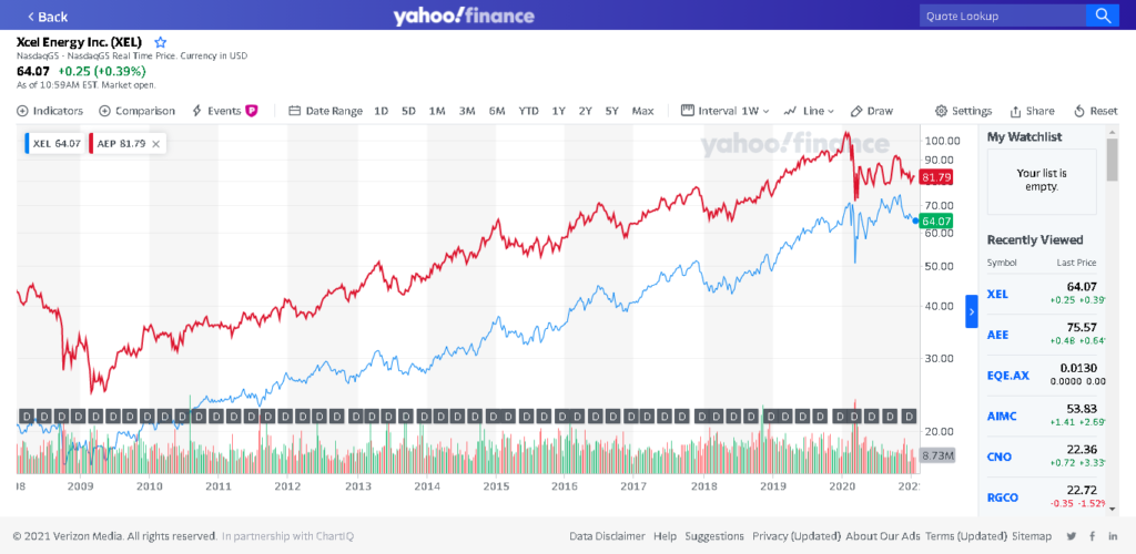
To determine the signal for when a trade should occur, we look at the difference between the two stocks:
In [22]: diff = table['XEL']-table['AEP']

In [23]: diff.mean()
Out[23]: -24.10590632758745

In [24]: diff.std()
Out[24]: 3.148618069119123
Now, we can say with a reasonably high level of confidence that if the two stocks diverge by more than 2 standard deviations (or ~ 6.3), there is a trading opportunity. Let’s see if that happens in the period following this one:
> next_period = df.pivot(columns='ticker')
> next_period.columns = [col[1] for col in next_period.columns]
> next_period.index = pd.to_datetime(next_period.index)

> next_period = next_period['2020-01-01':]
> next_diff = next_period['XEL']-next_period['AEP']
> next_diff.loc[next_diff < -30.4]
date
2020-01-15   -30.736753
2020-01-16   -30.877687
2020-01-17   -31.762922
2020-01-21   -31.903163
2020-01-22   -32.340503
2020-01-23   -32.607094
2020-01-24   -33.502785
2020-01-27   -33.378315
2020-01-28   -33.482761
2020-01-29   -33.890905
2020-01-30   -33.828830
2020-01-31   -33.521868
2020-02-03   -33.265412
2020-02-04   -32.095119
2020-02-05   -31.362759
2020-02-06   -30.806166
2020-02-07   -31.866599
2020-02-10   -32.091640
2020-02-11   -32.485245
2020-02-12   -31.993412
2020-02-13   -32.256399
2020-02-14   -32.717131
2020-02-18   -32.389837
2020-02-19   -31.938717
2020-02-20   -30.955869
So according to the pairs trading algorithm provided, we would open the trade on January 15, 2020 (XEL @ 63.59, AEP @ 94.33). The algorithm closes the trade when the two stocks cross their mean difference again. This happens on March 11, 2020 (XEL @ 65.90, AEP @ 88.21). This trade would therefore earn us $8.43, ignoring transaction costs.
A real test of the pairs trading algorithm
So in the one example, we did earn a positive return by following the pairs trading algorithm. The question is: does this generalize, and can we beat the market with this strategy? We will now look at a much larger number of correlated pairs.
First, we need to codify the trading algorithm. For readability, we will iterate over the DataFrames, although in practice there are much better ways to do this. We define a function to calculate per-trade profit
def calc_trade_profit(ticker1, ticker2, start_date, end_date):
    if next_period.loc[start_date][ticker1] > next_period.loc[start_date][ticker2]:
        high_ticker = ticker1
        low_ticker = ticker2

    else:
        high_ticker = ticker2
        low_ticker = ticker1

    short_profit = next_period.loc[start_date][high_ticker] - next_period.loc[end_date][high_ticker]
    long_profit = next_period.loc[end_date][low_ticker] - next_period.loc[start_date][low_ticker]

    return long_profit + short_profit
Now, we iterate over each day in the period. For each day, we will iterate over the correlated pairs to find whether they trade on that day. If the difference between the prices of the two stocks is greater than the threshold (and was less yesterday), we open the trade. If the trade is open, and the difference between the prices goes below the mean, we close the trade.
Here’s our code:
print("starting trades")
for index, row in next_period.iterrows():
    # iterate over the days of the next period

    for sindex, srow in corrdata.iterrows():
        # iterate over the correlated pairs

        ticker1 = sindex[0]
        ticker2 = sindex[1]

        trade = ticker1 + '-' + ticker2

        mean = srow['mean']
        std = srow['std']

        if not trade in trades:
            trades[trade] = { 'open' : False, 'start' : None, 'earned' : 0. }

        threshold = abs(mean) + 2*std
        print(trade + " " + str(row[ticker1]) + " " + str(row[ticker2]) + " " + str(threshold) + " " + str(abs(row[ticker1] - row[ticker2])))

        if ticker1 in prevrow:
            if abs(row[ticker1] - row[ticker2]) > threshold and abs(prevrow[ticker1] - prevrow[ticker2] <= threshold):
                #open a trade if not open
                if not trades[trade]['open']:
                    print("opening trade " + ticker1 + "-" + ticker2 + ": " + str(index))
                    trades[trade]['start'] = index
                    trades[trade]['open'] = True

            if abs(row[ticker1] - row[ticker2]) < abs(mean) and abs(prevrow[ticker1] - prevrow[ticker2]) >= abs(mean):
                #close an open trade
                if trades[trade]['open']:
                    print("closing trade " + ticker1 + "-" + ticker2 + ": " + str(index))
                    trades[trade]['earned'] = trades[trade]['earned'] + calc_trade_profit(ticker1, ticker2, trades[trade]['start'], index)
                    trades[trade]['start'] = None
                    trades[trade]['open'] = False

    prevrow = row
Finally, we need to close all open trades on the last day (these are the ones that may be losers):
#now close all of the open trades on the last day of the period
last_day = next_period.index[-1]

for sindex, srow in corrdata.iterrows():
    # iterate over the correlated pairs

    ticker1 = sindex[0]
    ticker2 = sindex[1]

    trade = ticker1 + '-' + ticker2
    if (trade in trades) and (trades[trade]['open']):
        print("last day: closing trade " + ticker1 + "-" + ticker2)
        trades[trade]['earned'] = trades[trade]['earned'] + calc_trade_profit(ticker1, ticker2, trades[trade]['start'], last_day)
        trades[trade]['start'] = None
        trades[trade]['open'] = False


print("total earned: " + str(functools.reduce(lambda acc,v: acc+trades[v]['earned'], trades, 0)))
Now, we run this algorithm on the top 100 correlated pairs:
XEL   AEP     0.996523
V     MA      0.994791
NEE   ETR     0.994646
WEC   XEL     0.994444
      CMS     0.994384
SUI   ELS     0.993536
CMS   XEL     0.993018
AWK   XEL     0.992827
UDR   AVB     0.992741
      AIV     0.992524
WEC   AWK     0.992214
HE    AEP     0.992158
SUI   ETR     0.991948
      MAA     0.991770
CMS   LNT     0.991266
ADC   O       0.991101
HE    XEL     0.991046
OPTT  FCEL    0.990808
AON   AJG     0.990615
WELL  PEAK    0.990414
AIV   AVB     0.990408
TRNO  PLD     0.990302
NEE   LNT     0.990216
AEP   AWK     0.989953
POR   AEP     0.989822
CMS   AEP     0.989687
O     AIV     0.989058
      UDR     0.989025
POR   XEL     0.988931
PEAK  O       0.988882
DRE   EGP     0.988872
SO    ETR     0.988799
DRE   FR      0.988766
AWK   AMT     0.988565
PNM   XEL     0.988536
HE    AWK     0.988447
ELS   ETR     0.988435
O     NNN     0.988409
EGP   ELS     0.988395
MSFT  V       0.988302
SUI   NEE     0.987992
CMS   POR     0.987979
CVV   BLIN    0.987850
OGE   AEE     0.987712
AEP   WEC     0.987688
CMS   AWK     0.987651
TRNO  SUI     0.987628
PEAK  ADC     0.987585
LNT   ETR     0.987326
AEP   PNM     0.987310
PEAK  UDR     0.987200
POR   AVB     0.987179
AVB   CPT     0.987089
EQR   ESS     0.986930
LNT   WEC     0.986684
USM   TDS     0.986674
WPC   PSB     0.986629
NWE   DTE     0.986558
CPT   EQR     0.986507
AEE   DTE     0.986407
XEL   AMT     0.986397
EGP   SUI     0.986270
ATO   CMS     0.986256
NEE   FE      0.986243
AEE   NWE     0.986101
CMS   EQR     0.986014
EGP   STWD    0.985946
MA    MSFT    0.985910
CMS   FE      0.985907
NWE   POR     0.985815
NEE   ELS     0.985728
CCI   AMT     0.985701
MT    HAL     0.985365
EQR   UDR     0.985344
MAA   ETR     0.985262
MPW   O       0.985165
EQR   AVB     0.985094
BAH   ARCC    0.984924
MA    FICO    0.984884
HE    WEC     0.984878
AEP   AMT     0.984747
SUI   SO      0.984630
NEE   SO      0.984616
WEC   ETR     0.984588
PNM   AWK     0.984569
FR    TRNO    0.984532
HE    PNM     0.984259
BKH   NWE     0.984165
STE   BAH     0.984014
AWR   WEC     0.983979
V     ARCC    0.983937
UDR   ADC     0.983922
MAA   TRNO    0.983697
PSB   WELL    0.983626
MAA   NEE     0.983566
VRSK  MSI     0.983533
BAH   V       0.983492
HE    AMT     0.983375
AWK   POR     0.983327
FE    LNT     0.983292
Results of the pairs trading algorithm
From the period of January 1, 2020 to August 18, 2020, the algorithm would have earned a profit of $284, by trading one long and one short share at each signal. Since each long is paired with a larger short, you could achieve this with essentially $0 initial investment (ignoring trading costs), making the return essentially infinite. Moreover, if you run the model from January 1, 2020 to April 1, 2020, you would have seen a significant profit, even while the S&P 500 had dropped by almost 25%.
However, in reality, whenever you open a short position, you assume a liability.
Conclusion: does pairs trading still work in 2021?
Our model shows that pairs trading can work and be profitable in 2021. The question of how profitable, and whether it is worth the risk is something we will tackle in a future article.
No Comments