
Beat the market using volume data: is it possible? [2022]
![Beat the market using volume data: is it possible? [2022]](https://firemymoneymanager.com/wp-content/uploads/2022/02/Figure_1-2-800x462.png)
In this article we will look at whether it is possible to predict a crash using historical market data.
Related reading
Before reading this article, it’s useful to understand the basics backtesting in Python. We recommend you read these:
- Getting started: using Python to find alpha [2021]
- Do Stocks Exhibit Momentum? A reality check [2021]
Can volume spikes predict a crash?
Let’s begin by looking at historical volume on a chart. Here we have QQQ, the Nasdaq ETF plotted from 2005 to today:
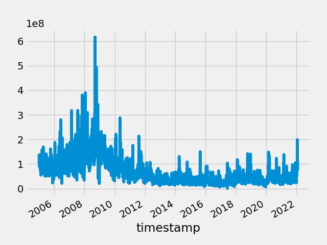
There are clearly volume spikes around major crashes (2008, 2020), but the magnitude of the spikes can very greatly.
Let’s try a backtest (using Python and bt), with a simple rule: if today’s volume is greater than 50 million, get out (or stay out) of the market. Otherwise be fully invested. Here is the code for this rule:
class TestBuyAlgo(bt.core.Algo):

    def __call__(self, target):
        if target.now in returns.index:
            if z.loc[target.now]['volume'] > 50000000:
                target.temp['selected'] = [t]
                target.temp['weights'] = {t:0}
            else:
                target.temp['selected'] = t
                target.temp['weights'] = { t:1 }

            return True
        return False


roa = TestBuyAlgo()
we = bt.algos.WeighEqually()
rb = bt.algos.Rebalance()

start = '2006-11-03'

spy = bt.Strategy(t, [bt.algos.SelectThese([t]),we,rb])
benchmark = bt.Backtest(
    spy,
    z[start:],
    integer_positions=False
)

strat = bt.Strategy('Mega', [roa,rb])
backtest = bt.Backtest(
    strat,
    z[start:],
    integer_positions=False
)

res = bt.run(backtest,benchmark)
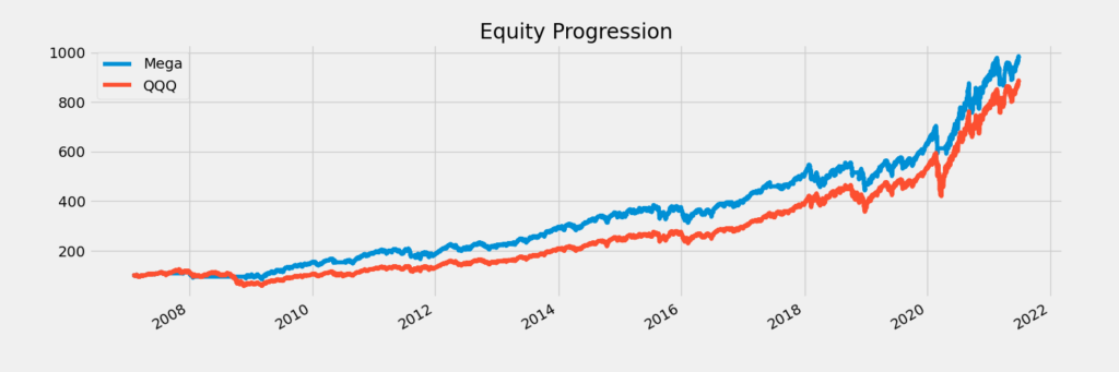
Here’s a plot of the result:
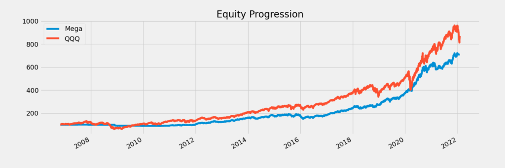
This backtest clearly underperforms in pure returns; however, when we look at the risk adjusted return, it actually performs rather well. It’s monthly Sortino ratio is almost double that of the QQQ ETF. Moreover, it almost completely bypasses both the 2020 crash and the 2008 crash. Here are the performance figures:
Stat                 Mega        QQQ
-------------------  ----------  ----------
Start                2006-11-02  2006-11-02
End                  2022-02-01  2022-02-01
Risk-free rate       0.00%       0.00%

Total Return         610.03%     771.74%
Daily Sharpe         1.17        0.76
Daily Sortino        1.81        1.20
CAGR                 13.72%      15.26%
Max Drawdown         -21.72%     -53.55%
Calmar Ratio         0.63        0.28

MTD                  0.00%       0.68%
3m                   3.83%       -5.66%
6m                   12.40%      0.26%
YTD                  -0.35%      -8.13%
1Y                   16.58%      13.37%
3Y (ann.)            34.60%      29.71%
5Y (ann.)            30.00%      23.86%
10Y (ann.)           20.48%      19.60%
Since Incep. (ann.)  13.72%      15.26%

Daily Sharpe         1.17        0.76
Daily Sortino        1.81        1.20
Daily Mean (ann.)    13.54%      16.61%
Daily Vol (ann.)     11.55%      21.84%
Daily Skew           -0.29       -0.15
Daily Kurt           10.19       8.35
Best Day             7.15%       12.16%
Worst Day            -7.52%      -11.98%

Monthly Sharpe       1.16        0.87
Monthly Sortino      2.54        1.54
Monthly Mean (ann.)  13.59%      15.58%
Monthly Vol (ann.)   11.72%      17.98%
Monthly Skew         0.32        -0.45
Monthly Kurt         1.42        0.71
Best Month           13.94%      14.97%
Worst Month          -10.28%     -15.63%

Yearly Sharpe        0.73        0.72
Yearly Sortino       6.94        1.60
Yearly Mean          14.45%      16.88%
Yearly Vol           19.69%      23.38%
Yearly Skew          1.46        -0.78
Yearly Kurt          2.40        1.50
Best Year            68.07%      53.83%
Worst Year           -8.31%      -41.94%

Avg. Drawdown        -1.84%      -2.60%
Avg. Drawdown Days   26.67       22.80
Avg. Up Month        3.60%       4.33%
Avg. Down Month      -1.36%      -4.08%
Win Year %           75.00%      81.25%
Win 12m %            73.99%      86.13%
Can we do better using moving averages of volume?
The naïve rule that we used worked pretty well, but if we look at the plot of volume, we can see that spikes in volume very much depend on the context, and that many of the non-crash days after 2008 had higher volumes than the crash of 2020.
It looks like we should be able to do better with higher resolution data, but can we? Let’s try using hourly data to see how well it works. Since hourly data is noisy, we want a way to smooth out the data a bit.
We first try a moving average. We take a 100 hour moving average period and compare it to a 1000 hour moving average, from which we get this plot:
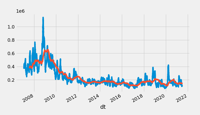
The spikes in this plot are adjusted volume spike events. Let’s look at the 100 hour volume divided by the 1000 hour volume:
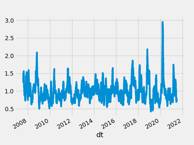
From this plot we can see that there are a small number of spikes over 1.5. Let’s try running a simulation in which we get out of the market when the 100 hour moving average is more than 1.5 times the 1000 hour moving average.
z = pd.read_csv("qqq.txt")
z['dt'] = pd.to_datetime(z['Date'] + ' ' + z['Time'].astype(str), format = "%m/%d/%Y %H%M")


z.index = pd.to_datetime(z['dt'])
z = z.sort_index()['2007-01-01':'2022-12-31']

daily_vol = z.groupby(z.index.date).agg({'Close':'last','Open':'first','Volume':'sum'}).reset_index()
daily_vol.index = pd.to_datetime(daily_vol['index'])

z = z.resample('H').last()
z = z.dropna()

returns = z['Close'].pct_change().dropna()*100
z = z.rename({'Close':t},axis=1)

z['vol_sma_100'] = z['Volume'].rolling(100).mean()
z['vol_sma_1000'] = z['Volume'].rolling(1000).mean()


class TestBuyAlgo(bt.core.Algo):

    def __init__(self):
        self.oom_date = None


    def __call__(self, target):

        if target.now in returns.index:

            loc = returns.index.get_loc(target.now)
            if loc < len(returns) - 2:

                today = returns.index[loc].date()

                if self.oom_date is not None:
                    if self.oom_date != today:
                        if z.index[loc].time().hour == 15:
                            if daily_vol.loc[pd.to_datetime(today)]['Volume'] < 50000000:
                                self.oom_date = None
                elif z.loc[target.now]['vol_sma_100'] > 1.5 * z.loc[target.now]['vol_sma_1000']:
                    target.temp['selected'] = [t]
                    target.temp['weights'] = {t:0}
                    print("out of market " + str(today))
                    self.oom_date = today
                else:
                    target.temp['selected'] = t
                    target.temp['weights'] = { t:1 }

                return True

        return False


roa = TestBuyAlgo()
we = bt.algos.WeighEqually()
rb = bt.algos.Rebalance()

start = '2007-02-07'
spy = bt.Strategy(t, [bt.algos.SelectThese([t]),we,rb])
benchmark = bt.Backtest(
    spy,
    z[start:],
    integer_positions=False
)

strat = bt.Strategy('Test', [roa,rb])
backtest = bt.Backtest(
    strat,
    z[start:],
    integer_positions=False
)

res = bt.run(backtest,benchmark)
When we run this simulation, we get a very good result:
Stat                 Mega        QQQ
-------------------  ----------  ----------
Start                2007-02-06  2007-02-06
End                  2021-06-25  2021-06-25
Risk-free rate       0.00%       0.00%

Total Return         881.85%     784.29%
Daily Sharpe         1.01        0.79
Daily Sortino        1.57        1.25
CAGR                 17.21%      16.36%
Max Drawdown         -25.53%     -53.31%
Calmar Ratio         0.67        0.31

MTD                  4.82%       4.82%
3m                   12.38%      12.38%
6m                   9.38%       13.18%
YTD                  7.96%       11.71%
1Y                   37.83%      42.62%
3Y (ann.)            24.57%      27.70%
5Y (ann.)            23.78%      28.90%
10Y (ann.)           17.70%      21.34%
Since Incep. (ann.)  17.21%      16.36%

Daily Sharpe         1.01        0.79
Daily Sortino        1.57        1.25
Daily Mean (ann.)    17.39%      17.65%
Daily Vol (ann.)     17.24%      22.25%
Daily Skew           -0.36       -0.15
Daily Kurt           4.25        9.17
Best Day             6.32%       12.63%
Worst Day            -7.41%      -12.58%

Monthly Sharpe       1.11        0.95
Monthly Sortino      2.14        1.70
Monthly Mean (ann.)  17.39%      17.07%
Monthly Vol (ann.)   15.60%      18.02%
Monthly Skew         -0.27       -0.48
Monthly Kurt         0.75        0.81
Best Month           13.00%      15.07%
Worst Month          -14.08%     -16.00%

Yearly Sharpe        0.94        0.76
Yearly Sortino       5.55        1.65
Yearly Mean          18.33%      18.36%
Yearly Vol           19.49%      24.19%
Yearly Skew          0.27        -0.87
Yearly Kurt          -0.69       1.92
Best Year            54.67%      54.67%
Worst Year           -11.44%     -41.75%

Avg. Drawdown        -2.27%      -2.45%
Avg. Drawdown Days   21.50       21.38
Avg. Up Month        4.20%       4.45%
Avg. Down Month      -2.76%      -3.95%
Win Year %           78.57%      85.71%
Win 12m %            85.80%      86.42%
No Comments