The basis for modern portfolio theory, as well as many quantitative strategies for investing or trading is that financial instruments — especially equities — follow a normal distribution. In our articles on finding alpha, CAPM, or even pairs trading, we assume a generally normal (but not necessarily perfectly normal) distribution.

But do they still do that in 2021? Did they ever do that? We will attempt to answer that question in this article.

How to identify a normal distribution

A normal distribution is a sample distribution that is roughly bell shaped. One of the most important characteristics of a normal distribution is that it is symmetrical around the center.

We can create a random normal distribution to see this using Python:

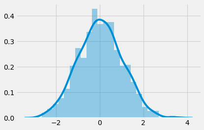
z = np.random.normal(size=1000)
sns.distplot(z)

The resulting plot shows the 1000 samples form this symmetrical bell curve shape:

But how do we determine that this is really a normal distribution? How do we quantify its normalness?

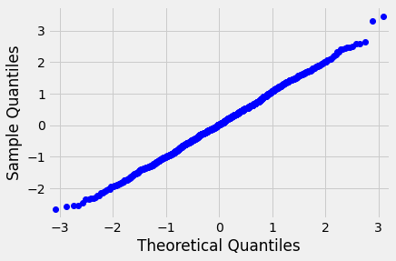
First, let’s look at a QQ plot. A QQ plot is a good way for visually determining normalness. We won’t go into the specifics of how it works, but a normal distribution should show up on the QQ plot as a straight line. Here is the plot of the above distribution:

But we need to do this for a lot of equities. How can we do this quantitatively? We can use a Kolmogorov-Smirnov test.

Here is how the NIST explains this test:

The Kolmogorov-Smirnov test is used to decide if a sample comes from a population with a specific distribution.

The Kolmogorov-Smirnov (K-S) test is based on the empirical distribution function (ECDF). Given N ordered data points Y₁, Y₂, …, Y_N, the ECDF is defined as

E_N=n(i)/N

where n(i) is the number of points less than Y_i and the Y_i are ordered from smallest to largest value. This is a step function that increases by 1/N at the value of each ordered data point.

Essentially, what this test tells us is the probability that one of the samples is in the red zone in the graph below (the zone that deviates from the normal distribution):

If the probability is large, that means that the data is not very normally distributed. If the probability is small, then the data is normally distributed. (Note that the way the actual test works is more complicated and beyond the scope of this article.)

Generally, people interpret the results as a normal distribution if the test returns more than .05. Let’s try this test on our sample data:

scipy.stats.kstest(rvs=z, cdf='norm')
Out[18]: KstestResult(statistic=0.021468169352233724, pvalue=0.737569346346318)

So the KS statistic is .73, which is far above our .05 cutoff. This is clearly a strong normal distribution.

Determining normal distribution for a stock

In order to determine whether equities follow this normal distribution, we need to load some data. We use Quandl data to load in equities on the NASDAQ or NYSE. For this test, we will also look at ETFs.

We use the following Python code to load the data (this code is based on the code we developed in Getting Started):

alldata = pd.DataFrame()


try: 
    ticker_data = pd.read_csv("tickers.csv")
except FileNotFoundError as e:
    pass


ticker_data = ticker_data.loc[((ticker_data['table'] == 'SF1')) & (ticker_data['isdelisted'] == 'N') & (ticker_data['currency'] == 'USD') & ((ticker_data.exchange == 'NYSE') | (ticker_data.exchange == 'NYSEMKT') | (ticker_data.exchange == 'NYSEARCA') | (ticker_data.exchange == 'NASDAQ'))]


for t in ticker_data['ticker']:
    if t == 'TRUE': continue
        
    print(t)
    
    try:
        data = pd.read_csv(t + ".csv", 
                            header = None,
                            usecols = [0, 1, 12],
                            names = ['ticker', 'date', 'adj_close'])
    
        if (len(data) < 2000): #ignore bad data (we have to look into wjhy)
            continue
        
        alldata = alldata.append(data)
        
    except FileNotFoundError as e:
        pass

df = alldata.set_index('date')
table = df.pivot(columns='ticker')
table.columns = [col[1] for col in table.columns]

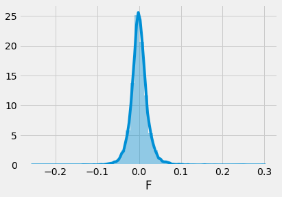
Now we can look at some distribution charts. Let’s try Ford (F) first. We clean the data by calculating percentage changes (for comparison) and droping N/A values.

ford = table['F'].pct_change().dropna()
sns.distplot(ford)

And here is the chart output. Looks pretty normal, right?

Now, let’s run the KS test on this distribution and determine how normal it actually is:

scipy.stats.kstest(rvs=ford, cdf='norm')
Out[16]: KstestResult(statistic=0.4686455878905682, pvalue=0.0)

Uh oh…why is it 0? The function uses the standard normal distribution. To tell it to use a different normal distribution, we have to add the mean and standard deviation as arguments:

scipy.stats.kstest(ford, 'norm', args=(ford.mean(),ford.std()))
Out[21]: KstestResult(statistic=0.07156629413923976, pvalue=1.3427916967898793e-54)

So the actual value is very small. This isn’t a normal distribution. The QQ plot makes this pretty clear:

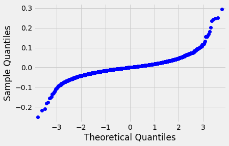
If this were a normal distribution, the plot would be linear; however, it’s much more of an S shape. We can remove the outliers to make it look more like a normal distribution, but it still doesn’t fit that well.

The tails of the plot show that the stock has more extreme values than the normal distribution would predict.

Determining normal distribution over all equities

In the last section, we found that Ford stock didn’t meet the criteria for a real normal distribution.

Now, we want to determine whether equities as a whole are normally distributed. So we will try to run the same code to get an average p-value for all equities in our dataset:

ks = pd.DataFrame(columns = ['ticker', 'ks', 'p'])
i = 0

for ticker in table.columns:
    pct_returns = table[ticker].pct_change().dropna()
    r = scipy.stats.kstest(pct_returns, 'norm', args=(pct_returns.mean(),pct_returns.std()))

    ks.loc[i] = [ticker, r.statistic, r.pvalue]
    i = i+1
    

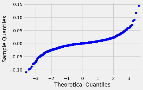
Running that code, we get an average p value that is significantly less than .05. Let’s look at a QQ plot of the S&P 500 ETF to understand how it diverges from a normal distribution:

Let’s do a sort on all of the KS p-values and see if there are any that show a true normal distribution:

     ticker        ks         p
2499   NVCN  0.374057  0.000000
612     CKX  0.291689  0.000000
2547    OEG  0.282855  0.000000
2055    LEU  0.300688  0.000000
1775   IKNX  0.251512  0.000000
    ...       ...       ...
3694   VGLT  0.037264  0.001079
3551    TYO  0.035553  0.001320
3639    UST  0.033326  0.005089
1751   IGOV  0.031124  0.006564
3606    UNL  0.025611  0.056922

[3937 rows x 3 columns]

So there are some tickers that do (just barely) meet the criteria for a normal distribution. However, these aren’t stocks. They’re treasury ETFs and other non-equity ETFs. The equity tickers are all under the threshold for a normal distribution.

Conclusion

From our analysis, it is clear that stocks returns don’t follow a totally normal distribution. The question we need to ask in the future is whether the distribution is sufficiently normal for modern portfolio theory to work. We will study that in other articles.