
Do CAPM efficient portfolios really outperform random ones? [2021]
![Do CAPM efficient portfolios really outperform random ones? [2021]](https://firemymoneymanager.com/wp-content/uploads/2021/08/plt-800x247.png)
How to create an efficient portfolio
One of the most basic tenets of Modern Portfolio Theory (which many professional investors still follow) is that each stock moves with the market in a certain, relatively constant, way (this applies to most financial instruments, but we will focus on stocks here). This is referred to as the beta of the stock.
By combining stocks into a portfolio, you get a linear function that can be optimized by standard optimization methods. More specifically, because each stock is a linear function of the market return, you get something like this:
Stock 1 return: α1 + β1(Rm – Rf) + ε1
Stock 2 return: α2 + β2(Rm – Rf) + ε2
and so on, where:
Rf is the risk-free return
αi is the stock’s alpha
βi is the stock’s beta
Rm is the market return
εi is a stochastic error term
When you combine these functions together, you get a total portfolio return, which can be rewritten like this:
α1 + α2+ … + αn + [ β1 + β2 + … + βn ](Rm – Rf) + ε
Modern Portfolio theory says that if we find beta values to maximize this function, and then use those beta values as weights in the portfolio, we can get an optimized, or “efficient” portfolio.
In this article, we will use Python to find efficient beta values each month, and then see if the returns from those efficient portfolios actually beat their value-weighted, equal weight, or randomly weighted alternatives.
Calculating beta values for an efficient portfolio
We load the data for this experiment the same way we did a previous article. We will use the bt package for Python to do the backtest simulation.
After the basic setup, we need to write functions to find the beta values for an efficient portfolio. Ricky Kim wrote an excellent article on portfolio optimization here. We won’t explain how all of this works — if you are interested, you can learn the details about it in the linked article.
We use Ricky Kim’s functions and modify them a bit to operate on our data:
def portfolio_annualised_performance(weights, mean_returns, cov_matrix):
    returns = np.sum(mean_returns*weights ) *252
    std = np.sqrt(np.dot(weights.T, np.dot(cov_matrix, weights))) * np.sqrt(252)

    return std, returns

def neg_sharpe_ratio(weights, mean_returns, cov_matrix, risk_free_rate):
    p_var, p_ret = portfolio_annualised_performance(weights, mean_returns, cov_matrix)
    return -(p_ret - risk_free_rate) / p_var

def max_sharpe_ratio(mean_returns, cov_matrix, risk_free_rate):
    num_assets = len(mean_returns)
    args = (mean_returns, cov_matrix, risk_free_rate)
    constraints = ({'type': 'eq', 'fun': lambda x: np.sum(x) - 1})
    bound = (0.0,1.0)
    bounds = tuple(bound for asset in range(num_assets))
    result = sco.minimize(neg_sharpe_ratio, num_assets*[1./num_assets,], args=args,
                        method='SLSQP', bounds=bounds, constraints=constraints)
    return result

def display_ef_with_selected(mean_returns, cov_matrix, risk_free_rate, ctable):
    max_sharpe = max_sharpe_ratio(mean_returns, cov_matrix, risk_free_rate)
    print(max_sharpe)
    sdp, rp = portfolio_annualised_performance(max_sharpe['x'], mean_returns, cov_matrix)
    max_sharpe_allocation = pd.DataFrame(max_sharpe.x,index=ctable.columns,columns=['allocation'])
    max_sharpe_allocation.allocation = [round(i*100,2)for i in max_sharpe_allocation.allocation]
    max_sharpe_allocation = max_sharpe_allocation.T
    return max_sharpe_allocation
It is not necessary to understand how the code above works, except that the function display_ef_with_selected takes a table of returns, a covariance matrix, the risk free interest rate, and a table of returns by ticker.
Simulating the returns of the efficient portfolio vs. alternatives
Next, we write the code to buy and rebalance the most efficient grouping on a monthly basis. We will create three separate functions for bt to simulate: the efficient portfolio, a market-cap-weighted portfolio, and a randomly weighted portfolio.
Let’s first create the function for the randomly weighted portfolio. There are better ways to do this in pandas, but our intention is to make the code as straightforward to read as possible.
class RandomWeightedMegacapAlgo(bt.core.Algo):


    def __call__(self, target):


        if target.now in mtable.index:

            i0 = table.index.get_loc(target.now)
            iprev = i0 - 1
            dprev = table.index[iprev].strftime('%Y-%m-%d')

            mc = get_megacap(dprev)
            weights = {}

            if len(mc) == 0:
                return True

            mytickers = []

            m = daily.query('`date`==@dprev')
            m = m.sort_values('marketcap', ascending=False)

            if (len(m) > 0):
                for i in range(0, len(mc)):
                    z = m.iloc[i]
                    if z['ticker'] in table:
                        weights[z['ticker']] = random.random()
                        mytickers.append(z['ticker'])

            total_weight = sum(weights.values())
            target.temp['selected'] = mytickers
            target.temp['weights'] = { key: value/total_weight for key,value in weights.items() }


            return True

        return False
The function above will act only monthly (even though we have daily data), and will first select all stocks that we define as mega-cap ($100B or more). It defines a random weight for each ticker.
Next, we create the function for the market-cap-weighted portfolio:
class MCWeightedMegacapAlgo(bt.core.Algo):


    def __call__(self, target):

        #act monthly on daily data
        if target.now in mtable.index:


            #get the last months data
            i0 = table.index.get_loc(target.now)
            iprev = i0 - 1
            dprev = table.index[iprev].strftime('%Y-%m-%d')

            # get mega cap
            mc = get_megacap(dprev)
            caps = {}

            if len(mc) == 0:
                return True

            mytickers = []

            m = daily.query('`date`==@dprev')
            m = m.sort_values('marketcap', ascending=False)

            if (len(m) > 0):
                for i in range(0, len(mc)):
                    z = m.iloc[i]
                    if z['ticker'] in table:
                        caps[z['ticker']] = z['marketcap']
                        mytickers.append(z['ticker'])

            total_cap = sum(caps.values())
            if total_cap == 0:
                target.temp['selected'] = []
                target.temp['weights'] = {}
            else:
                target.temp['selected'] = mytickers
                target.temp['weights'] = { key: value/total_cap for key,value in caps.items() }


            return True

        return False
This function operates like the previous one, except that it finds the market caps for each stock from the daily DataFrame and sets the target.temp weight values according to market cap.
The equally weighted function is similar to the function above:
class EqualWeightedMegacapAlgo(bt.core.Algo):


    def __call__(self, target):


        if target.now in mtable.index:
            print(target.now)
            i0 = table.index.get_loc(target.now)
            iprev = i0 - 1
            dprev = table.index[iprev].strftime('%Y-%m-%d')

            mc = get_megacap(dprev)
            weights = {}

            if len(mc) == 0:
                return True

            mytickers = []

            m = daily.query('`date`==@dprev')
            m = m.sort_values('marketcap', ascending=False)

            if (len(m) > 0):
                for i in range(0, len(mc)):
                    z = m.iloc[i]
                    if z['ticker'] in table:
                        weights[z['ticker']] = 1
                        mytickers.append(z['ticker'])

            total_weight = sum(weights.values())
            target.temp['selected'] = mytickers
            target.temp['weights'] = { key: value/total_weight for key,value in weights.items() }


            return True

        return False
Finally, we write the function for the efficient portfolio. Again, this function could be optimized, but for the sake of clarity we will sacrifice some speed.
 class OptimizedMegacapAlgo(bt.core.Algo):


    def __call__(self, target):


        if target.now in mtable.index:
            i0 = table.index.get_loc(target.now)
            iprev = i0 - 1
            dprev = table.index[iprev].strftime('%Y-%m-%d')

            mc = get_megacap(dprev)

            if len(mc) == 0:
                return True

            ctable = table[:dprev][mc]

            r = ctable.pct_change()
            mean_returns = r.mean()
            cov = r.cov()
            msa = display_ef_with_selected(mean_returns, cov, .01, ctable)

            selected = []
            weights = {}

            for s in msa.columns:
                selected.append(s)
                weights[s] = msa[s].allocation/100

            target.temp['weights'] = weights
            target.temp['selected'] = selected

            return True

        return False
How does this function work? Every month (at the end of the month), it gets the largest stocks (just like above) and then calculates the mean and covariance of the daily returns for these stocks. We use the data from the previous month in order to avoid data snooping.
Then, the function calls display_ef_with_selected, which returns the most efficient allocation of the stocks — the weighting of stocks that results in the maximum Sharpe ratio (mean returns divided by standard deviation). Note that we pass a table of values up to the previous month, again to avoid data snooping.
Finally, the function sets the weights of the stocks based on the calculated efficient weights.
Do optimized efficient portfolios outperform alternatives?
We can now get to the question of whether the optimization we performed actually resulted in better performance.
We run the back test from 2017 to mid-2020 and get these results:
Stat                 Equal       Random      Market Cap    Efficient    SPY         QQQ
-------------------  ----------  ----------  ------------  -----------  ----------  ----------
Start                2017-01-30  2017-01-30  2017-01-30    2017-01-30   2017-01-30  2017-01-30
End                  2020-08-18  2020-08-18  2020-08-18    2020-08-18   2020-08-18  2020-08-18
Risk-free rate       0.00%       0.00%       0.00%         0.00%        0.00%       0.00%

Total Return         53.41%      48.60%      78.34%        64.86%       59.22%      129.85%
Daily Sharpe         0.70        0.65        0.89          0.78         0.74        1.13
Daily Sortino        1.02        0.95        1.32          1.15         1.09        1.71
CAGR                 12.82%      11.81%      17.71%        15.13%       14.01%      26.44%
Max Drawdown         -32.15%     -32.21%     -30.37%       -31.69%      -33.70%     -28.56%
Calmar Ratio         0.40        0.37        0.58          0.48         0.42        0.93

MTD                  4.40%       3.79%       4.87%         5.95%        3.71%       4.58%
3m                   13.43%      11.56%      17.32%        24.86%       15.30%      22.43%
6m                   0.58%       -0.90%      8.04%         13.02%       1.63%       18.88%
YTD                  4.30%       1.55%       14.09%        27.46%       6.33%       31.25%
1Y                   15.52%      12.47%      28.45%        40.20%       19.61%      51.07%
3Y (ann.)            12.07%      10.98%      17.45%        16.50%       13.93%      26.36%
5Y (ann.)            -           -           -             -            -           -
10Y (ann.)           -           -           -             -            -           -
Since Incep. (ann.)  12.82%      11.81%      17.71%        15.13%       14.01%      26.44%

Daily Sharpe         0.70        0.65        0.89          0.78         0.74        1.13
Daily Sortino        1.02        0.95        1.32          1.15         1.09        1.71
Daily Mean (ann.)    14.11%      13.23%      18.49%        16.32%       15.22%      26.19%
Daily Vol (ann.)     20.15%      20.26%      20.79%        21.00%       20.48%      23.28%
Daily Skew           -0.82       -0.81       -0.61         -0.90        -0.78       -0.59
Daily Kurt           20.43       21.08       18.06         20.79        18.15       11.46
Best Day             8.90%       9.56%       9.70%         9.31%        9.06%       8.47%
Worst Day            -11.58%     -11.79%     -11.53%       -12.33%      -10.94%     -11.98%

Monthly Sharpe       0.90        0.84        1.14          0.98         0.91        1.45
Monthly Sortino      1.43        1.34        1.94          1.88         1.43        2.80
Monthly Mean (ann.)  13.05%      12.12%      17.40%        15.20%       14.28%      24.89%
Monthly Vol (ann.)   14.56%      14.36%      15.29%        15.47%       15.74%      17.19%
Monthly Skew         -0.76       -0.69       -0.54         -0.20        -0.82       -0.38
Monthly Kurt         1.50        1.61        1.41          -0.09        2.07        0.71
Best Month           11.35%      11.61%      13.41%        12.15%       12.70%      14.97%
Worst Month          -10.38%     -10.17%     -9.09%        -8.21%       -12.46%     -8.65%

Yearly Sharpe        0.58        0.51        0.84          0.65         0.60        1.13
Yearly Sortino       4.45        3.97        10.01         2.24         4.18        348.02
Yearly Mean          9.45%       8.29%       14.45%        13.80%       11.00%      23.36%
Yearly Vol           16.32%      16.35%      17.14%        21.25%       18.34%      20.70%
Yearly Skew          1.28        1.54        0.10          -1.70        1.07        -1.47
Yearly Kurt          -           -           -             -            -           -
Best Year            27.72%      26.93%      31.78%        27.46%       31.22%      38.96%
Worst Year           -3.68%      -3.62%      -2.50%        -10.68%      -4.56%      -0.12%

Avg. Drawdown        -1.58%      -1.65%      -1.51%        -2.58%       -1.62%      -2.27%
Avg. Drawdown Days   15.85       17.05       13.32         29.51        15.84       14.18
Avg. Up Month        2.88%       2.69%       3.23%         3.73%        2.99%       4.47%
Avg. Down Month      -4.83%      -5.35%      -5.27%        -3.84%       -5.62%      -4.10%
Win Year %           66.67%      66.67%      66.67%        66.67%       66.67%      66.67%
Win 12m %            93.94%      93.94%      93.94%        78.79%       93.94%      96.97%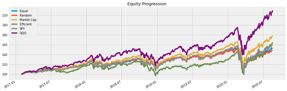
Here we see that the efficient portfolio underperforms compared to the market-cap weighted portfolio on a risk-adjusted basis. However, it does outperform compared to the random and equal weight portfolios.
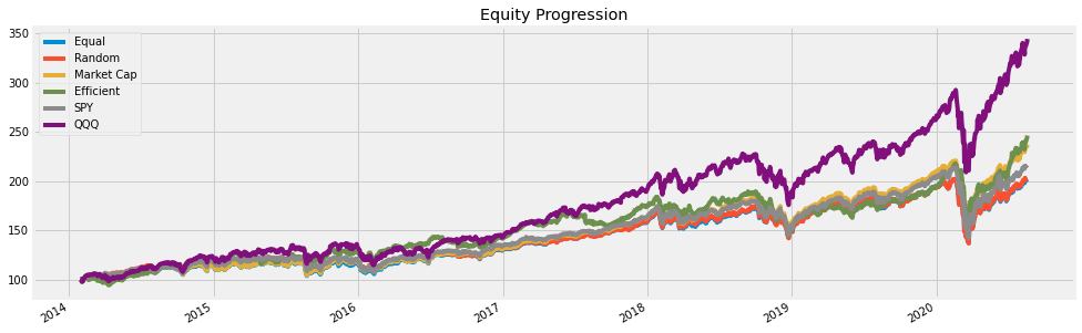
Let’s look at a longer term and see if the same holds true:
Stat                 Equal       Random      Market Cap    Efficient    SPY         QQQ
-------------------  ----------  ----------  ------------  -----------  ----------  ----------
Start                2014-01-30  2014-01-30  2014-01-30    2014-01-30   2014-01-30  2014-01-30
End                  2020-08-18  2020-08-18  2020-08-18    2020-08-18   2020-08-18  2020-08-18
Risk-free rate       0.00%       0.00%       0.00%         0.00%        0.00%       0.00%

Total Return         101.83%     102.61%     137.11%       146.07%      116.15%     244.23%
Daily Sharpe         0.71        0.71        0.83          0.85         0.76        1.04
Daily Sortino        1.06        1.06        1.27          1.29         1.14        1.60
CAGR                 11.32%      11.38%      14.09%        14.74%       12.49%      20.77%
Max Drawdown         -32.15%     -32.45%     -30.37%       -31.69%      -33.70%     -28.56%
Calmar Ratio         0.35        0.35        0.46          0.47         0.37        0.73

MTD                  4.40%       4.09%       4.87%         5.95%        3.71%       4.58%
3m                   13.43%      13.07%      17.32%        24.86%       15.30%      22.43%
6m                   0.58%       0.78%       8.04%         13.02%       1.63%       18.88%
YTD                  4.30%       4.85%       14.09%        27.46%       6.33%       31.25%
1Y                   15.52%      14.93%      28.45%        40.20%       19.61%      51.07%
3Y (ann.)            12.07%      12.22%      17.45%        16.50%       13.93%      26.36%
5Y (ann.)            11.66%      11.03%      15.18%        14.87%       12.25%      21.29%
10Y (ann.)           -           -           -             -            -           -
Since Incep. (ann.)  11.32%      11.38%      14.09%        14.74%       12.49%      20.77%

Daily Sharpe         0.71        0.71        0.83          0.85         0.76        1.04
Daily Sortino        1.06        1.06        1.27          1.29         1.14        1.60
Daily Mean (ann.)    12.24%      12.32%      14.78%        15.42%       13.33%      20.95%
Daily Vol (ann.)     17.29%      17.45%      17.74%        18.13%       17.53%      20.23%
Daily Skew           -0.75       -0.70       -0.55         -0.82        -0.73       -0.55
Daily Kurt           21.18       20.30       19.24         20.85        19.09       11.66
Best Day             8.90%       8.89%       9.70%         9.31%        9.06%       8.47%
Worst Day            -11.58%     -11.33%     -11.53%       -12.33%      -10.94%     -11.98%

Monthly Sharpe       0.91        0.91        1.06          1.08         0.94        1.28
Monthly Sortino      1.53        1.54        1.91          2.14         1.57        2.61
Monthly Mean (ann.)  11.51%      11.57%      14.05%        14.67%       12.68%      20.14%
Monthly Vol (ann.)   12.70%      12.67%      13.27%        13.63%       13.52%      15.79%
Monthly Skew         -0.53       -0.50       -0.28         -0.07        -0.61       -0.14
Monthly Kurt         1.69        1.78        1.58          0.18         2.27        0.42
Best Month           11.35%      11.66%      13.41%        12.15%       12.70%      14.97%
Worst Month          -10.38%     -10.16%     -9.09%        -8.21%       -12.46%     -8.65%

Yearly Sharpe        0.89        0.84        1.09          0.96         0.85        1.22
Yearly Sortino       7.15        5.93        13.44         3.15         6.09        418.88
Yearly Mean          10.74%      10.25%      13.73%        13.72%       11.32%      19.88%
Yearly Vol           12.02%      12.17%      12.61%        14.34%       13.29%      16.30%
Yearly Skew          0.43        0.50        0.27          -1.04        0.49        -0.05
Yearly Kurt          -1.33       -1.21       -0.85         0.57         -0.79       -2.54
Best Year            27.72%      27.62%      31.78%        27.46%       31.22%      38.96%
Worst Year           -3.68%      -4.24%      -2.50%        -10.68%      -4.56%      -0.12%

Avg. Drawdown        -1.57%      -1.68%      -1.61%        -2.29%       -1.55%      -2.23%
Avg. Drawdown Days   16.63       17.70       15.40         25.61        16.34       16.09
Avg. Up Month        2.67%       2.70%       2.90%         3.46%        2.77%       4.25%
Avg. Down Month      -3.46%      -3.26%      -3.59%        -2.85%       -3.68%      -3.27%
Win Year %           83.33%      83.33%      83.33%        83.33%       83.33%      83.33%
Win 12m %            91.30%      88.41%      91.30%        88.41%       91.30%      92.75%
In this case, the efficient portfolio generally does outperform its alternatives on a risk adjusted basis. Here is the chart:
We can also backtest with a different set of stocks (market cap $50B to $100B). Again, the optimized efficient portfolio is not the best risk adjusted performer.
Stat                 Equal       Random      Market Cap    Efficient    SPY         QQQ
-------------------  ----------  ----------  ------------  -----------  ----------  ----------
Start                2018-01-30  2018-01-30  2018-01-30    2018-01-30   2018-01-30  2018-01-30
End                  2020-08-18  2020-08-18  2020-08-18    2020-08-18   2020-08-18  2020-08-18
Risk-free rate       0.00%       0.00%       0.00%         0.00%        0.00%       0.00%

Total Return         21.91%      18.53%      37.98%        36.52%       26.06%      67.50%
Daily Sharpe         0.45        0.40        0.64          0.63         0.50        0.89
Daily Sortino        0.66        0.60        0.97          0.96         0.74        1.37
CAGR                 8.08%       6.89%       13.46%        12.99%       9.51%       22.43%
Max Drawdown         -32.06%     -32.33%     -30.32%       -34.20%      -33.70%     -28.56%
Calmar Ratio         0.25        0.21        0.44          0.38         0.28        0.79

MTD                  4.22%       3.97%       4.77%         2.11%        3.71%       4.58%
3m                   13.16%      13.44%      17.14%        9.88%        15.30%      22.43%
6m                   0.53%       0.70%       7.83%         3.73%        1.63%       18.88%
YTD                  4.28%       3.58%       13.90%        14.18%       6.33%       31.25%
1Y                   15.57%      13.21%      28.28%        23.79%       19.61%      51.07%
3Y (ann.)            8.08%       6.89%       13.46%        12.99%       9.51%       22.43%
5Y (ann.)            -           -           -             -            -           -
10Y (ann.)           -           -           -             -            -           -
Since Incep. (ann.)  8.08%       6.89%       13.46%        12.99%       9.51%       22.43%

Daily Sharpe         0.45        0.40        0.64          0.63         0.50        0.89
Daily Sortino        0.66        0.60        0.97          0.96         0.74        1.37
Daily Mean (ann.)    10.56%      9.48%       15.57%        15.11%       11.94%      23.82%
Daily Vol (ann.)     23.50%      23.62%      24.14%        23.99%       23.77%      26.65%
Daily Skew           -0.65       -0.57       -0.50         -0.37        -0.66       -0.52
Daily Kurt           14.71       13.11       13.16         19.63        13.23       8.67
Best Day             8.95%       8.77%       9.75%         9.89%        9.06%       8.47%
Worst Day            -11.52%     -11.09%     -11.50%       -12.92%      -10.94%     -11.98%

Monthly Sharpe       0.54        0.47        0.80          0.78         0.58        1.13
Monthly Sortino      0.88        0.75        1.38          1.39         0.93        2.16
Monthly Mean (ann.)  9.04%       8.04%       14.01%        13.56%       10.63%      21.95%
Monthly Vol (ann.)   16.61%      17.20%      17.50%        17.33%       18.20%      19.41%
Monthly Skew         -0.52       -0.41       -0.38         -0.06        -0.60       -0.29
Monthly Kurt         0.43        0.68        0.40          1.79         0.86        0.09
Best Month           11.29%      12.35%      13.23%        15.05%       12.70%      14.97%
Worst Month          -10.16%     -10.48%     -8.98%        -11.15%      -12.46%     -8.65%

Yearly Sharpe        0.96        0.92        1.78          1.75         1.07        6.43
Yearly Sortino       inf         inf         inf           inf          inf         inf
Yearly Mean          16.32%      15.38%      23.04%        23.82%       18.78%      35.10%
Yearly Vol           17.03%      16.69%      12.93%        13.63%       17.60%      5.46%
Yearly Skew          -           -           -             -            -           -
Yearly Kurt          -           -           -             -            -           -
Best Year            28.36%      27.17%      32.18%        33.46%       31.22%      38.96%
Worst Year           4.28%       3.58%       13.90%        14.18%       6.33%       31.25%

Avg. Drawdown        -2.84%      -2.74%      -2.26%        -2.94%       -2.69%      -3.40%
Avg. Drawdown Days   25.94       25.52       18.34         25.56        23.49       19.24
Avg. Up Month        3.37%       3.20%       3.63%         3.49%        3.55%       4.92%
Avg. Down Month      -4.75%      -5.51%      -5.90%        -4.65%       -5.62%      -4.66%
Win Year %           100.00%     100.00%     100.00%       100.00%      100.00%     100.00%
Win 12m %            90.48%      85.71%      90.48%        85.71%       90.48%      95.24%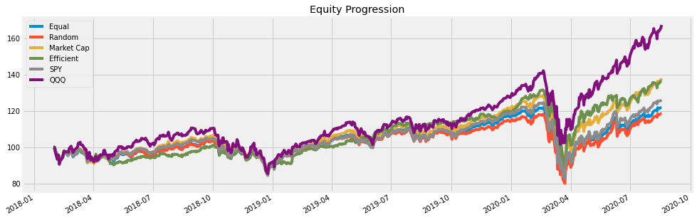
So, how did the efficient portfolio do?
Although the efficient portfolio did reasonably well compared to the random, equal, and market-cap weighted alternatives, it did not always perform the best. In fact, it was outperformed by the market-cap weighted portfolio two out of three times.
But perhaps we can do better. Let’s try to find the efficient portfolio by maximizing the Sortino ratio instead of the Sharpe ratio. The Sortino ratio differs from the Sharpe ratio in that it only divides by downward deviations from the benchmark, so it doesn’t penalize upward movements in a stock.
Let’s change the code to maximize the Sortino ratio:
def portfolio_annualised_performance(weights, mean_returns, cov_matrix, ctable, bench):
    #sortino
    p_returns = np.dot(ctable,weights)
    p_returns = p_returns[1:]
    bench = bench[1:]
    sp_returns = [0] * len(p_returns)

    for i in range(0,len(p_returns)):
        sp_returns[i] = ((p_returns[i] - bench[i]) if (p_returns[i] - bench[i] < 0) else 0)

    avg_return = np.mean(p_returns)
    std = np.std(sp_returns)
    return std*np.sqrt(252), avg_return*252

def neg_sharpe_ratio(weights, mean_returns, cov_matrix, risk_free_rate, ctable, bench):
    p_var, p_ret = portfolio_annualised_performance(weights, mean_returns, cov_matrix, ctable, bench)
    return -(p_ret - risk_free_rate) / p_var

def max_sharpe_ratio(mean_returns, cov_matrix, risk_free_rate, ctable, bench):
    num_assets = len(mean_returns)
    args = (mean_returns, cov_matrix, risk_free_rate, ctable, bench)
    constraints = ({'type': 'eq', 'fun': lambda x: np.sum(x) - 1})
    bound = (0.0,1.0)
    bounds = tuple(bound for asset in range(num_assets))
    result = sco.minimize(neg_sharpe_ratio, num_assets*[1./num_assets,], args=args,
                        method='SLSQP', bounds=bounds, constraints=constraints)
    return result

def display_ef_with_selected(mean_returns, cov_matrix, risk_free_rate, ctable, bench):
    max_sharpe = max_sharpe_ratio(mean_returns, cov_matrix, risk_free_rate, ctable, bench)

    sdp, rp = portfolio_annualised_performance(max_sharpe['x'], mean_returns, cov_matrix, ctable, bench)
    max_sharpe_allocation = pd.DataFrame(max_sharpe.x,index=ctable.columns,columns=['allocation'])
    max_sharpe_allocation.allocation = [round(i*100,2)for i in max_sharpe_allocation.allocation]
    max_sharpe_allocation = max_sharpe_allocation.T
    return max_sharpe_allocation
And we change OptimizedMegacapAlgo to pass in the benchmark. Since we are comparing the efficient portfolio to alternatives, let’s use the equal weighted portfolio as the benchmark.
And here are the results:
Stat                 Efficient    Equal       Random      Market Cap    SPY         QQQ
-------------------  -----------  ----------  ----------  ------------  ----------  ----------
Start                2015-02-01   2015-02-01  2015-02-01  2015-02-01    2015-02-01  2015-02-01
End                  2021-05-28   2021-05-28  2021-05-28  2021-05-28    2021-05-28  2021-05-28
Risk-free rate       0.00%        0.00%       0.00%       0.00%         0.00%       0.00%

Total Return         145.49%      114.13%     114.79%     144.24%       134.76%     246.10%
Daily Sharpe         0.86         0.77        0.76        0.86          0.84        1.02
Daily Sortino        1.30         1.15        1.15        1.30          1.25        1.58
CAGR                 15.27%       12.81%      12.86%      15.18%        14.46%      21.71%
Max Drawdown         -30.55%      -32.16%     -31.87%     -30.40%       -33.70%     -28.56%
Calmar Ratio         0.50         0.40        0.40        0.50          0.43        0.76

MTD                  -0.21%       1.78%       1.76%       -0.20%        0.66%       -1.20%
3m                   9.49%        10.96%      11.20%      9.50%         10.79%      6.43%
6m                   13.74%       15.20%      16.65%      13.72%        16.38%      12.02%
YTD                  9.19%        11.41%      12.31%      9.20%         12.71%      6.57%
1Y                   39.65%       37.42%      41.00%      39.32%        40.88%      46.10%
3Y (ann.)            20.09%       16.51%      16.87%      19.96%        18.20%      26.49%
5Y (ann.)            18.69%       15.65%      16.16%      18.60%        17.13%      25.90%
10Y (ann.)           -            -           -           -             -           -
Since Incep. (ann.)  15.27%       12.81%      12.86%      15.18%        14.46%      21.71%

Daily Sharpe         0.86         0.77        0.76        0.86          0.84        1.02
Daily Sortino        1.30         1.15        1.15        1.30          1.25        1.58
Daily Mean (ann.)    15.94%       13.63%      13.72%      15.85%        15.15%      21.96%
Daily Vol (ann.)     18.58%       17.72%      17.94%      18.53%        18.12%      21.46%
Daily Skew           -0.57        -0.78       -0.74       -0.57         -0.73       -0.54
Daily Kurt           16.83        19.70       19.75       16.69         17.24       9.58
Best Day             9.72%        8.83%       9.30%       9.69%         9.06%       8.47%
Worst Day            -11.58%      -11.60%     -11.67%     -11.54%       -10.94%     -11.98%

Monthly Sharpe       1.06         0.95        0.96        1.05          0.97        1.20
Monthly Sortino      2.00         1.69        1.71        1.99          1.69        2.53
Monthly Mean (ann.)  15.51%       13.20%      13.23%      15.43%        14.10%      20.44%
Monthly Vol (ann.)   14.67%       13.93%      13.75%      14.66%        14.59%      16.97%
Monthly Skew         -0.11        -0.30       -0.37       -0.11         -0.40       0.00
Monthly Kurt         0.85         1.09        1.04        0.85          1.61        0.13
Best Month           13.38%       11.31%      10.88%      13.37%        12.70%      14.97%
Worst Month          -9.09%       -10.39%     -10.43%     -9.10%        -12.46%     -8.65%

Yearly Sharpe        1.29         1.32        1.17        1.29          1.27        1.10
Yearly Sortino       16.72        9.78        5.21        16.30         8.19        469.77
Yearly Mean          16.53%       14.01%      14.49%      16.44%        15.24%      22.30%
Yearly Vol           12.78%       10.61%      12.43%      12.76%        11.96%      20.29%
Yearly Skew          -0.41        -0.67       -0.95       -0.40         -0.60       0.19
Yearly Kurt          -1.21        0.78        1.09        -1.19         1.29        -2.39
Best Year            31.30%       26.92%      27.48%      31.28%        31.22%      48.62%
Worst Year           -2.42%       -3.51%      -6.82%      -2.47%        -4.56%      -0.12%

Avg. Drawdown        -1.72%       -1.71%      -1.62%      -1.64%        -1.53%      -2.49%
Avg. Drawdown Days   15.82        18.33       18.54       16.02         15.58       16.94
Avg. Up Month        3.20%        3.06%       3.06%       3.19%         3.03%       4.45%
Avg. Down Month      -3.95%       -3.61%      -3.61%      -3.96%        -3.93%      -3.47%
Win Year %           83.33%       83.33%      83.33%      83.33%        83.33%      83.33%
Win 12m %            93.85%       93.85%      92.31%      93.85%        92.31%      92.31%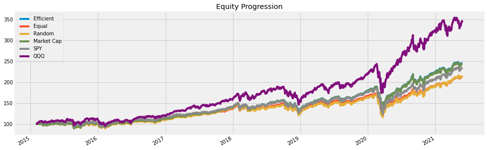
Stat                 Efficient    Equal       Random      Market Cap    SPY         QQQ
-------------------  -----------  ----------  ----------  ------------  ----------  ----------
Start                2015-02-01   2015-02-01  2015-02-01  2015-02-01    2015-02-01  2015-02-01
End                  2015-12-31   2015-12-31  2015-12-31  2015-12-31    2015-12-31  2015-12-31
Risk-free rate       0.00%        0.00%       0.00%       0.00%         0.00%       0.00%

Total Return         1.01%        -0.12%      0.85%       1.20%         3.07%       10.81%
Daily Sharpe         0.15         0.07        0.14        0.16          0.29        0.72
Daily Sortino        0.24         0.11        0.22        0.26          0.47        1.17
CAGR                 1.11%        -0.13%      0.93%       1.31%         3.37%       11.92%
Max Drawdown         -13.39%      -12.79%     -12.34%     -13.40%       -11.91%     -13.94%
Calmar Ratio         0.08         -0.01       0.08        0.10          0.28        0.85

MTD                  -1.03%       -0.72%      -0.42%      -1.00%        -1.72%      -1.59%
3m                   8.89%        8.14%       8.53%       8.93%         7.03%       10.29%
6m                   2.79%        1.58%       2.70%       2.83%         0.16%       5.06%
YTD                  1.01%        -0.12%      0.85%       1.20%         3.07%       10.81%
1Y                   -            -           -           -             -           -
3Y (ann.)            -            -           -           -             -           -
5Y (ann.)            -            -           -           -             -           -
10Y (ann.)           -            -           -           -             -           -
Since Incep. (ann.)  1.11%        -0.13%      0.93%       1.31%         3.37%       11.92%

Daily Sharpe         0.15         0.07        0.14        0.16          0.29        0.72
Daily Sortino        0.24         0.11        0.22        0.26          0.47        1.17
Daily Mean (ann.)    2.31%        1.03%       2.08%       2.50%         4.44%       12.73%
Daily Vol (ann.)     15.60%       15.27%      15.29%      15.56%        15.27%      17.79%
Daily Skew           -0.13        -0.21       -0.15       -0.13         -0.28       -0.12
Daily Kurt           2.92         2.60        2.44        2.93          2.62        2.90
Best Day             4.26%        3.86%       3.90%       4.26%         3.84%       5.04%
Worst Day            -3.93%       -4.01%      -3.86%      -3.92%        -4.21%      -4.37%

Monthly Sharpe       0.15         0.05        0.13        0.16          -0.05       0.37
Monthly Sortino      0.30         0.10        0.25        0.33          -0.10       0.84
Monthly Mean (ann.)  2.17%        0.77%       1.84%       2.38%         -0.67%      6.30%
Monthly Vol (ann.)   14.73%       14.36%      13.65%      14.67%        13.33%      17.23%
Monthly Skew         0.75         0.60        0.40        0.75          0.96        0.99
Monthly Kurt         1.71         1.57        1.26        1.70          2.43        1.85
Best Month           9.23%        8.68%       8.06%       9.21%         8.51%       11.39%
Worst Month          -6.62%       -6.83%      -6.58%      -6.57%        -6.10%      -6.82%

Yearly Sharpe        -            -           -           -             -           -
Yearly Sortino       -            -           -           -             -           -
Yearly Mean          -            -           -           -             -           -
Yearly Vol           -            -           -           -             -           -
Yearly Skew          -            -           -           -             -           -
Yearly Kurt          -            -           -           -             -           -
Best Year            -            -           -           -             -           -
Worst Year           -            -           -           -             -           -

Avg. Drawdown        -3.48%       -3.40%      -3.39%      -3.47%        -2.27%      -3.13%
Avg. Drawdown Days   36.25        41.57       32.33       36.25         30.10       22.77
Avg. Up Month        3.26%        3.02%       3.02%       3.26%         2.68%       4.15%
Avg. Down Month      -2.89%       -2.89%      -2.72%      -2.87%        -2.79%      -3.10%
Win Year %           -            -           -           -             -           -
Win 12m %            -            -           -           -             -           -
Again, the efficient portfolio allocation is not always the best, but it does tend to perform pretty well. That said, the market-cap weighted portfolio almost always outperforms it.
Conclusion: do efficient portfolios outperform alternatives?
From the results we can see that efficient portfolios do perform relatively well, but you will always do just as well or better with a market-cap weighted portfolio.
tl;dr:
- Does a CAPM optimized efficient portfolio outperform a market-cap weighted portfolio? No, in general you’re likely to do just as well or better with a market-cap weighted portfolio. It doesn’t seem to make sense to optimize a portfolio beyond using a market-cap weighted.
- Does a CAPM optimized efficient portfolio outperform a randomly weighted portfolio? Yes, in general it does.
- Does a CAPM optimized efficient portfolio outperform an equally weighted portfolio? Yes, in general it does.
No Comments