In this article, we get started examining the CAPM and Fama/French alphas by calculating their values for real stocks. Understanding this procedure allows us to build on these models in other articles.

Basu and Fama/French provided important methods for modeling excess returns based on factors beyond the standard Capital Asset Pricing Model. Unfortunately, not all of their papers are easily available online. However, there are plenty of summaries of their work, which are useful reading.

The basis for alpha: related reading

The following papers do a good job in summarizing the work of Basu and Farma/French, and they have the added benefit of being freely available online:

• Investment Performance and Price-Earnings Ratios: Basu 1977 Revisited
• Investment Performance of Common Stock in Relation to their Price-Earnings Ratios
• The Volatility Effect: Lower Risk without Lower Return
• Five Concerns with the Five-Factor Model
• Minimum-Variance Portfolios in the U.S. Equity Market

The concepts of alpha and beta assume that equities follow a normal distribution. We look into whether that is true in this article.

Step 1: loading the data using Pandas

Let’s look at Russell 2000 stocks. These should give us a good dataset with which we can work.

We begin by loading in all of the data from Quandl, using the list of Russell 2000 stocks.

import pandas as pd  
import numpy as np
import matplotlib.pyplot as plt
import seaborn as sns
import quandl
import pickle
import csv
from datetime import date
import sys
import statsmodels.api as sm
import scipy.optimize as sco
plt.style.use('fivethirtyeight')
np.random.seed(777)



pd.set_option('display.max_rows', 100)
pd.set_option('display.max_columns', 100)


tickers = []
used_tickers = []

with open("russell2000tick.csv") as csvfile:
    reader = csv.reader(csvfile)
    for row in reader:
        tickers.append(row[0])
    
alldata = pd.DataFrame()

for ticker in tickers:

    try:
        data = pd.read_csv("stockdata/" + ticker + ".csv", 
                            header = None,
                            usecols = [0, 1, 12],
                            names = ['ticker', 'date', 'adj_close'])
    
        alldata = alldata.append(data)
        used_tickers.append(ticker)
        print(ticker)
        
    except FileNotFoundError as e:
        pass

tickers = used_tickers

Now, we can get a table with columns for each ticker and date rows:

df = alldata.set_index('date')
table = df.pivot(columns='ticker')
table.columns = [col[1] for col in table.columns]

Step 2: Cleaning the data for analysis

There are a lot of NaN values in this dataset, so we can clean them out by first removing columns with more than 30 NaNs. Holidays also have NaN values, so we need to remove the dates with holidays. We can do this by adding this code:

table = table['2010-01-04':'2020-08-18']

# we want the percentage change for comparison
table = table.pct_change()
table = table.loc[:, (table.isnull().sum(axis=0) <= 30)]
table = table.dropna(axis='rows')

Now, we are ready to find the CAPM α and β.

Step 3: Alpha and the CAPM equation

The basic CAPM equation is

R_i – R_f = α_i + β_i(R_m – R_f) + ε_i

Where

R_i is the return on the stock in the given time period

R_f is the risk-free return

α_i is the CAPM alpha

β_i is the CAPM beta

R_m is the market return

ε_i is a stochastic error term

Determining CAPM market return and risk free rates

Fama and French (from the paper linked above) keep a data library with calculations of the market return and risk free rate, which can be accessed from here.

The CSV doesn’t have a header for the first column, so we edit the header and name the first column ‘Date’. Then we can load and format the CSV like this:

factors = pd.read_csv("famafactors.csv")
factors['Date'] = pd.to_datetime(factors['Date'],format='%Y%m%d')
factors['Mkt-RF'] = factors['Mkt-RF'] / 100
factors = factors.set_index('Date')

Now, we combine the factors and the returns tables:

factors = factors['2010-01-04':'2020-08-18']
table = factors.merge(table, left_index=True, right_index=True, how='inner')

Step 4: Running regressions to find alpha

At this point, it’s easy to plot regression lines for individual stocks. If we want to see a plot for NL, we can do this:

sns.regplot(y='Mkt-RF', x='NL', data=table)

Now, we can start running correlations. For the first test, we will do a regression on the daily data. This will obviously result in a low correlation, due to the amount of noise in the data. However, it gives us a baseline from which we can do further analysis.

To do this, we use the following code:

regressions = pd.DataFrame(columns = ['ticker', 'alpha', 'beta', 'rsquared'])

# start at 6 to skip date and fama factors
for i in range(6, len(table.columns)):
    
    # for calculating y, we must subtract the risk free rate
    y = table[table.columns[i]] - table['_RF']
    X = table['Mkt-RF']

    ro = y.between(y.quantile(.01), y.quantile(.99))
    y = y[ro]
    X = X[ro]
    
    X = sm.add_constant(X)
    
   
    model = sm.OLS(y, X).fit()
    
    regressions.loc[i-6] = [ 
        table.columns[i],
        model.params['const'],
        model.params['Mkt-RF'],
        model.rsquared
    ]
                    

Note that we filtered out outliers here that are in the top or bottom 1%. It’s up to you whether you think that makes sense in this particular context.

For a sanity check we can first run the regressions against a list of ETFs. This should give us the broader market ETFs (S&P 500 ETFs for example) first, and they should be nearly 100% correlated to the Mkt-RF. Here is the output:

124    CORP -0.002448  0.000005  1.215519e-10
1008    SHY -0.002567 -0.000072  5.407849e-08
505    IBND -0.002573  0.000222  1.326580e-07
758     NOM -0.002519  0.001175  9.270459e-07
653     LQD -0.002432  0.000688  2.020755e-06
    ...       ...       ...           ...
1071    SSO -0.002655  1.920029  9.420202e-01
1060   SPXS -0.002690 -2.859140  9.637690e-01
1061   SPXU -0.002657 -2.854800  9.639438e-01
1059   SPXL -0.002696  2.873916  9.641320e-01
1134   UPRO -0.002690  2.881056  9.644571e-01

As you can see, the best correlated are UPRO and SPXL, which are both triple-long S&P 500 ETFs. The beta for both of these tickers is nearly 3, which makes sense. SPXS, the triple-short S&P 500 ETF, is next, with a beta of -3. And at the bottom, we have a corporate bond ETF.

Now, we can return to using stock tickers. After running the code again, regressions is a table of all tickers with their daily alpha, beta, and r-squared factors. We can sort it to get the most well correlated and the least well correlated tickers:

     ticker     alpha      beta      rsquared
1015    GFI -0.002056  0.003114  8.205919e-07
2578   WHLM -0.002060 -0.009481  6.090840e-06
650     CVR -0.002334  0.006751  1.254616e-05
1948   PRPH -0.001908  0.010896  1.521615e-05
2355    THM -0.002350 -0.019028  1.782250e-05
    ...       ...       ...           ...
32      ACN -0.002495  0.974155  5.241445e-01
843      EV -0.002993  1.272874  5.278900e-01
2401   TROW -0.002700  1.121679  5.570539e-01
132     AMP -0.002748  1.392772  5.767456e-01
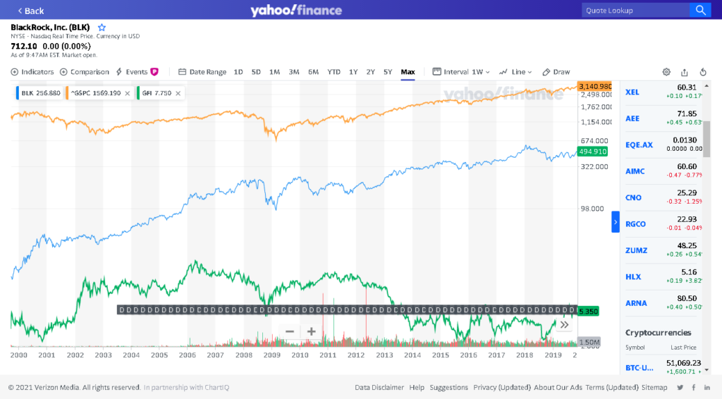
337     BLK -0.002516  1.229884  5.860815e-01

You can see that the least correlated ticker is GFI, which is Gold Fields Limited, one of the largest gold mining firms. Obviously, gold related instruments are going to move very differently from most equities. The most closely correlated is BlackRock.

We can look at these on a chart (the S&P 500 is in orange, BlackRock is in blue, and GFI is in green):

Resampling to Monthly

Running these regressions on daily data may be interesting, but not particularly useful. Due to the error inherent in CAPM, we need to look at longer time periods. So we now resample the data to monthly.

First, we load the monthly factor data, which is in a slightly different format.

factors = pd.read_csv("d:\\famafactorsmonthly.csv")
factors['Date'] = pd.to_datetime(factors['Date'],format='%Y%m')
factors['Mkt-RF'] = factors['Mkt-RF'] / 100
factors = factors.set_index('Date')

The monthly factor data is the data from the end of each month. Unfortunately, this loads the monthly data on the first of each month. So we need to change the dates to end of month:

factors.index = factors.index.to_period('M').to_timestamp('M')

Now, we can run the ETF test again on the monthly time scale. And here are our results:

     ticker     alpha      beta  rsquared
1012    SJB -0.059726  0.005377  0.000010
96      CCZ -0.049075 -0.020540  0.000076
426    GDXJ -0.066987  0.096735  0.000570
753     NMI -0.053687  0.055460  0.000775
1266    YCL -0.065084  0.057360  0.000893
    ...       ...       ...       ...
1105   TQQQ -0.051655  3.366393  0.625342
1131   UMDD -0.068596  3.494975  0.648961
684    MIDU -0.069756  3.542325  0.658577
1059   SPXL -0.061149  3.023759  0.666595
1134   UPRO -0.060995  3.033314  0.667091

SJB is a short bond ETF, so it makes sense that it would be uncorrelated to equities. Meanwhile, we see the same ETFs at the top of the list.

Now, let’s look at the list of equities, this time sorting by alpha:

     ticker     alpha      beta  rsquared
2380   TOPS -0.209049  1.177885  0.028528
448     CEI -0.189496  1.496256  0.035676
684    DCTH -0.184497  0.085347  0.000182
1012   GEVO -0.184126  2.639587  0.261636
1709   NSPR -0.181267  2.010658  0.112558
    ...       ...       ...       ...
784    EHTH -0.008732 -0.119886  0.000704
2306    TAL -0.006959  0.486709  0.023229
847     EVI -0.006877  0.974036  0.030031
1253   INSG -0.004456  1.306819  0.047048
728      DQ -0.003193  1.698251  0.076006

So here we go, the alphas of all stocks — and there’s one thing we notice immediately: they’re all less than 0.

Testing the Fama-French Model

One thing we learn from this is that the CAPM model is not a very good fit for current stock prices. When we run a regression, our r-squared value maxes out at less than .5 for non-ETFs, meaning the fit is not very good.

There is another popular and more recent model called the Fama-French model. This model adds additional variables to the CAPM equation. The Fama-French equation is:

The Fama-French equation is

R_i – R_f = α_i + β_i(R_m – R_f) + s_pSMB + h_pHML + ε_i

Where the alpha, beta, and epsilon terms remain the same, but two new terms are added:

s_pSMB, which is a variable s_p multiplied by a precalculated value of the difference between small and big portfolios

h_pHML, which is a variable h_p multiplied by a precalculated value of the difference between the highest book to market ratio and the lowest.

The creators of this model publish the values of HML and SMB at the link above.

Conclusion

There we have it, we have used Python and Pandas to find alphas for each stock in our dataset. From here, we can start looking into using these values for strategies, such as Mean-Variance Optimization, and basic statistical arbitrage.